1. Introduction
Warning
This manual refers to the ‘Vlieg’ calculation available in Diffcalc I. By default Diffcalc II now uses its ‘You’ engine. This manual will be updated soon. For now the developer guide shows how the new constraint system works.
This manual assumes that you are running Diffcalc within the external framework of the GDA or Minigda and that Diffcalc has been configured for the six circle diffractometer pictured here:
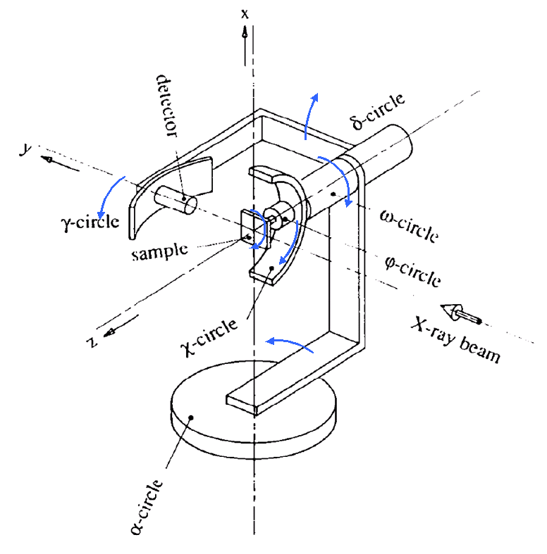
Gamma-on-delta six-circle diffractometer, modified from Elias Vlieg & Martin Lohmeier (1993)
Your Diffcalc configuration will have been customised for the geometry of your diffractometer and possibly the types of experiment you perform. For example: a five-circle diffractometer might be missing the Gamma circle above, some six-circle modes and the option to fix gamma that would otherwise exist in some modes.
The laboratory, crystal and reciprocal-lattice coordinate frames are defined with respect to the beam and to gravity to be (for a cubic crystal):

Laboratory and illustratrive crystal coordinate frames for a cubic crystal
The crystal lattice basis vectors are defined within the Cartesian crystal coordinate frame to be:
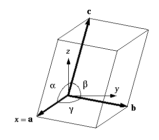
Unit cell defined in crystal coordinate frame
2. Overview
The following assumes that the diffractometer has been properly levelled, aligned with the beam and zeroed. See the SPEC fourc manual.
Before moving in hkl space you must calculate a UB matrix by specifying the crystal’s lattice parameters (which define the B matrix) and finding two reflections (from which the U matrix can be inferred); and, optionally for surface-diffraction experiments, determine how the surface of the crystal is oriented with respect to the phi axis.
Once a UB matrix has been calculated, the diffractometer may be driven in hkl coordinates. A valid diffractometer setting maps easily into a single hkl value. However for a diffractometer with more than three circles there are excess degrees of freedom when calculating a diffractometer setting from an hkl value. Diffcalc provides modes for using up the excess degrees of freedom.
Diffcalc does not perform scans directly. Instead, scannables that use diffcalc to map between reciprocal lattice space and real diffractometer settings are scanned using the Gda’s (or minigda’s) generic scan mechanism.
2.1. Theory
Thanks to Elias Vlieg for sharing his dos based DIF software that
Diffcalc has borrowed heavily from. (See also the THANKS.txt file).
See the papers (included in docs/ref):
- Busing & Levi (1966), “Angle Calculations for 3- and 4- Circle X-ray and Neutron Diffractometers”, Acta Cryst. 22, 457
- Elias Vlieg & Martin Lohmeier (1993), “Angle Calculations for a Six-Circle Surface X-ray Diffractometer”, J. Appl. Cryst. 26, 706-716
3. Getting Help
There are few commands to remember. If a command is called without arguments, Diffcalc will prompt for arguments and provide sensible defaults which can be chosen by pressing enter.
The helpub and helphkl commands provide help with the crystal
orientation and hkl movement phases of an experiment respectively:
>>> helpub

      Diffcalc
      --------
        helpub  ['command']        - lists all ub commands, or one if command is given
       helphkl  ['command']        - lists all hkl commands, or one if command is given

      UB State
      --------
         newub  'name'             - starts a new ub calculation with no lattice or
                                     reflection list
        loadub  'name'             - loads an existing ub calculation: lattice and
                                     reflection list
      saveubas  'name'             - saves the ubcalculation with a new name (other
                                     changes autosaved)
            ub                     - shows the complete state of the ub calculation

    UB lattice
    ----------
        setlat                     - prompts user to enter lattice parameters (in
                                     Angstroms and Deg.)
        setlat  'name' a           - assumes cubic
        setlat  'name' a b         - assumes tetragonal
        setlat  'name' a b c       - assumes ortho
        setlat  'name' a b c gam   - assumes mon/hex with gam not equal to 90
        setlat  'name' a b c alpha beta gamma  - arbitrary

    UB surface
    ----------
        sigtau  [sigma tau]        - sets sigma and tau

UB reflections
--------------
       showref                     - shows full reflection list
        addref                     - add reflection
        addref  h k l ['tag']      - add reflection with hardware position and energy
        addref  h k l (p1,p2...pN) energy ['tag']- add reflection with specified position
                                                   and energy
        delref  num                - deletes a reflection (numbered from 1)
       swapref                     - swaps first two reflections used for calculating U
       swapref  num1 num2          - swaps two reflections (numbered from 1)

UB calculation
--------------
          setu  [((,,),(,,),(,,))] - manually set u matrix
         setub  ((,,),(,,),(,,))   - manually set ub matrix
        calcub                     - (re)calculate u matrix from ref1 and ref2
       checkub                     - show calculated and entered hkl values for reflections

>>> helphkl

      Diffcalc
      --------
       helphkl  [command]          - lists all hkl commands, or one if command is given
        helpub  [command]          - lists all ub commands, or one if command is given

      Settings
      --------
       hklmode  [num]              - changes mode or shows current and available modes
                                     and all settings
      setalpha  [num]              - fixes alpha, or shows all settings if no num given
      setgamma  [num]              - fixes gamma, or shows all settings if no num given
     setbetain  [num]              - fixes betain, or shows all settings if no num given
    setbetaout  [num]              - fixes betaout, or shows all settings if no num given
    trackalpha  [boolean]          - determines wether alpha parameter will track alpha axis
    trackgamma  [boolean]          - determines wether gamma parameter will track gamma axis
      trackphi  [boolean]          - determines wether phi parameter will track phi axis
  setsectorlim  [omega_high omega_low phi_high phi_low]- sets sector limits

        Motion
        ------
           pos   hkl [h k l]       - move diffractometer to hkl, or read hkl position.
                                     Use None to hold a value still
           sim  hkl [h k l]        - simulates moving hkl
           hkl                     - shows loads of info about current hkl position
           pos  sixc [alpha, delta, gamma, omega, chi, phi,]- move diffractometer to Eularian
                                                              position. Use None to hold a
                                                              value still
           sim  sixc [alpha, delta, gamma, omega, chi, phi,]- simulates moving sixc
          sixc                     - shows loads of info about current sixc position
4. Diffcalc’s Scannables
Please see Moving in hkl space and Scanning in hkl space for some relevant examples.
To list and show the current positions of your beamline’s scannables
use pos with no arguments:
>>> pos
Results in:
Energy and wavelength scannables:
energy    12.3984
wl:       1.0000
Diffractometer scannables, as a group and in component axes (in the real GDA these have limits):
sixc:     alpha: 0.0000 delta: 0.0000 gamma: 0.0000 omega: 0.0000 chi: 0.0000 phi: 0.0000
alpha:    0.0000
chi:      0.0000
delta:    0.0000
gamma:    0.0000
omega:    0.0000
phi:      0.0000
Dummy counter, which in this example simply counts at 1hit/s:
cnt: 0.0000
Hkl scannable, as a group and in component:
hkl:      Error: No UB matrix
h:        Error: No UB matrix
k:        Error: No UB matrix
l:        Error: No UB matrix
Parameter scannables, used in some modes, these provide a
scannable alternative to the series of fix commands described in
Moving in hkl space.:
   alpha_par:0.00000
   azimuth:  ---
   betain:   ---
   betaout:  ---
   gamma_par:0.00000
   phi_par:  ---

Note that where a parameter corresponds with a physical
diffractometer axis, it can also be set to track that axis
directly. See `Tracking axis`_ below.
5. Crystal orientation
Before moving in hkl space you must calculate a UB matrix by specifying the crystal’s lattice parameters (which define the B matrix) and finding two reflections (from which the U matrix can be inferred); and, optionally for surface-diffraction experiments, determine how the surface of the crystal is oriented with respect to the phi axis (see Overview).
5.1. Starting a UB calculation
A UB-calculation contains the description of the crystal-under-test, any saved reflections, sigma & tau (both default to 0), and a B & UB matrix pair if they have been calculated or manually specified. Starting a new UB calculation will clear all of these.
Before starting a UB-calculation, the ub command used to summarise
the state of the current UB-calculation, will reflect that no
UB-calculation has been started:
>>> ub
No UB calculation started.
Wavelength: 1.239842
    Energy: 10.000000
A new UB-calculation calculation may be started and lattice specified explicitly:
>>> newub 'b16_270608'
>>> setlat 'xtal' 3.8401 3.8401 5.43072 90 90 90
or interactively:
>>> newub
calculation name: b16_270608
crystal name: xtal
       a [1]: 3.8401
  b [3.8401]: 3.8401
  c [3.8401]: 5.43072
  alpha [90]: 90
   beta [90]: 90
  gamma [90]: 90
where a,b and c are the lengths of the three unit cell basis vectors in Angstroms, and alpha, beta and gamma the typically used angles (defined in the figure above) in Degrees.
The ub command will show the state of the current UB-calculation
(and the current energy for reference):
UBCalc:     b16_270608
======

Crystal
-------
name:          xtal

lattice:                   a ,b ,c  =  3.84010,  3.84010,  5.43072
               alpha, beta , gamma  = 90.00000, 90.00000, 90.00000

reciprocal:             b1, b2, b3  =  1.63620,  1.63620,  1.15697
               beta1, beta2, beta3  =  1.57080,  1.57080,  1.57080

B matrix:      1.6362035642769  -0.0000000000000   -0.000000000000
               0.0000000000000   1.6362035642769   -0.000000000000
               0.0000000000000   0.0000000000000    1.156970955450

Reflections
-----------
energy h    k    l     alpha    delta    gamma    omega    chi      phi       tag

UB matrix
---------
none calculated

Sigma: 0.000000
Tau:   0.000000
Wavelength: 1.000000
Energy:    12.398420
5.2. Specifying Sigma and Tau for surface diffraction experiments
Sigma and Tau are used in modes that fix either the beam exit or entry angle with respect to the crystal surface, or that keep the surface normal in the horizontal laboratory plane. For non surface-diffraction experiments these can safely be left at zero.
For surface diffraction experiments, where not only the crystal’s lattice planes must be oriented appropriately but so must the crystal’s optical surface, two angles _Tau_ and _Sigma_ define the orientation of the surface with respect to the phi axis. Sigma is (minus) the amount of chi axis rotation and Tau (minus) the amount of phi axis rotation needed to move the surface normal parallel to the omega circle axis. These angles are often determined by reflecting a laser from the surface of the Crystal onto some thing and moving chi and tau until the reflected spot remains stationary with movements of omega.
Use sigtau with no args to set interactively:
>>> pos chi -3.1
chi:      -3.1000
>>> pos phi 10.0
phi:      10.0000
>>> sigtau
sigma, tau = 0.000000, 0.000000
  chi, phi = -3.100000, 10.000000
sigma[  3.1]: 3.1
  tau[-10.0]: 10.0
Sigma and Tau can also be set explicitly:
>>>sigtau 0 0
5.3. Managing reflections
The normal way to calculate a UB matrix is to find the position of two reflections with known hkl values. Diffcalc allows many reflections to be recorded but currently only uses the first two when calculating a UB matrix.
5.3.1. Add reflection at current location
It is normal to first move to a reflection:
>>> pos en 10
en:       10.0000
>>> pos sixc [5.000, 22.790, 0.000, 1.552, 22.400, 14.255]
sixc:     alpha: 5.0000 delta: 22.7900 gamma: 0.0000 omega: 1.5520 chi: 22.4000 phi: 14.2550
and then use the addref command either explicitly:
addref 1 0 1.0628 'optional_tag'
or interactively:
>>> addref
h: 1
k: 0
l: 1.0628
current pos[y]: y
tag: 'tag_string'
to add a reflection.
5.3.2. Add a reflection manually
If a reflection cannot be reached but its position is known (or if its position has been previously determined), a reflection may be added without first moving to it either explicitly:
>>> addref 0 1 1.0628 [5.000, 22.790, 0.000,4.575, 24.275, 101.320] 'optional_tag'
or interactively:
>>> addref
h: 0
k: 1
l: 1.0628
current pos[y]: n
  alpha[5.000]:
  delta[22.79]:
  gamma[0.000]:
  omega[1.552]: 4.575
    chi[22.40]: 24.275
    phi[14.25]: 101.320
     en[9.998]:
    tag: optional_tag2
5.3.3. Edit reflection list
Use showref to show the reflection list:
>>> showref
     energy h    k    l     alpha    delta    gamma    omega    chi      phi       tag
  1  9.999  1.00 0.00 1.06  5.0000   22.7900  0.0000   1.5520   22.4000  14.2550   1st
  2  9.999  0.00 1.00 1.06  5.0000   22.7900  0.0000   4.5750   24.2750  101.32000 2nd
Use swapref to swap reflections:
>>> swapref 1 2
Recalculating UB matrix.
>>> showref
      energy h    k    l     alpha    delta    gamma    omega    chi      phi       tag
   1  9.999  0.00 1.00 1.06  5.0000   22.7900  0.0000   4.5750   24.2750  101.3200  2nd
   2  9.999  1.00 0.00 1.06  5.0000   22.7900  0.0000   1.5520   22.4000  14.2550   1st
Use delref to delete a reflection:
>>> delref 1
>>> showref
      energy h    k    l     alpha    delta    gamma    omega    chi      phi       tag
   1  9.999  1.00 0.00 1.06  5.0000   22.7900  0.0000   1.5520   22.4000  14.2550   1st
5.4. Calculating a UB matrix
Unless a U or UB matrix has been manually specified, a new UB matrix will be calculated after the second reflection has been found, or whenever one of the first two reflections is changed.
Use the command calcub to force the UB matrix to be calculated
from the first two reflections.
If you have misidentified a reflection used for the orientation the
resulting UB matrix will be incorrect. Always use the checkub
command to check that the computed values agree with the estimated values:
>>>checkub
   energy h    k    l     h_comp k_comp l_comp  tag
1  9.9987 1.00 0.00 1.06  1.0000 0.0000 1.0628  1st
2  9.9987 0.00 1.00 1.06 -0.0329 1.0114 1.0400  2nd
Notice that the first reflection will always match, but that the second will not match exactly. (The system of equations used to calculate the U matrix is overdetermined and some information from the second reflection is thrown away.)
5.5. Manually setting U and UB
To help find the initial reflections it may be useful to set the U
matrix manually—to the identity matrix for example. Use the setu
command to do this. Once set the diffractometer may be driven to the
ideal location of a reflection and then the actual reflection
sought. Normally this would be done in the default mode, four-circle-bisecting, (see
Moving in hkl space). In the following example this has been done
by setting the alpha to 5 and leaving gamma at 0 (it would be normal
to leave alpha at 0):
>>> hklmode 1
1) fourc bisecting
   alpha: 0.0
   gamma: 0.0

>>> setalpha 5
alpha: 0 --> 5.000000
>>> setu
row1[1 0 0]:
row2[0 1 0]:
row3[0 0 1]:
>>> sim hkl [1,0,1.0628] # Check it all makes sense
sixc would move to:
   alpha :   5.00000 deg
   delta :  22.79026 deg
   gamma :   0.00000 deg
   omega :   5.82845 deg
     chi :  24.57658 deg
     phi :   6.14137 deg

   theta : 70702.991919
  2theta : 23.303705
     Bin : 6.969151
    Bout : 6.969151
 azimuth : 7.262472

>>> pos hkl [1,0,1.0628]
hkl:      h: 1.00000 k: 0.00000 l: 1.06280

>>> # scan about to find actual reflection

>>> addref
h[0.0]: 1
k[0.0]: 0
l[0.0]: 1.0628
current pos[y]: y
tag: 'ref1'
>>>
There is currently no way to refine a manually specified U matrix by inferring as much as possible from just one found reflection.
6. Moving in hkl space
Once a UB matrix has been calculated, the diffractometer may be driven in hkl coordinates. A given diffractometer setting maps easily into a single hkl value. However for a diffractometer with more than three circles there are excess degrees of freedom when calculating a diffractometer setting from an hkl value. Diffcalc provides many for using up the excess degrees of freedom.
By default Diffcalc selects four-circle bisecting mode (see below).
Note that to play along with the following run the file in
example/session/sixc_example.py to configure the UB-calculation.
6.1. Modes
Use the command hklmode to summarise the state of Diffcalc’s angle
calculator. It shows a list the available modes for your
diffractometer and the parameters that must be fixed for each, the
current mode and the current parameter settings:
>>> hklmode
Available modes:
 0) fourc fixed-bandlw (alpha, gamma, blw) (Not impl.)
 1) fourc bisecting (alpha, gamma)
 2) fourc incoming  (alpha, gamma, betain)
 3) fourc outgoing  (alpha, gamma, betaout)
 4) fourc azimuth   (alpha, gamma, azimuth) (Not impl.)
 5) fourc fixed-phi (alpha, gamma, phi) (Not impl.)
10) fivec bisecting (gamma)
11) fivec incoming  (gamma, betain)
12) fivec outgoing  (gamma, betaout)
13) fivec bisecting (alpha)
14) fivec incoming  (alpha, betain)
15) fivec outgoing  (alpha, betaout)
20) zaxis bisecting ()
21) zaxis incoming  (betain)
22) zaxiz outgoing  (betaout)

Current mode:

1) fourc bisecting
Parameters:

   alpha: 0.0
   gamma: 0.0
  betain: --- (not relevant in this mode)
 betaout: --- (not relevant in this mode)
 azimuth: --- (not relevant in this mode)
     phi: --- (not relevant in this mode)
     blw: --- (not relevant in this mode)
Note that ‘Not impl.’ is short for ‘not implemented’. Standby.
Your output may differ. For example:
- When listed with a typical five-circle diffractometer with no gamma circle: the fourc modes will have no gamma parameter to fix (actually it will have been fixed under the covers to 0), there will be no gamma or alpha parameters to fix in the five circle modes (again, under the covers gamma will have been fixed) and there will be no zaxis modes (as these require six circles, or an actual z-axis diffractometer).
- When listed with a typical four-circle diffractometer with no alpha or gamma circle, the four-circle modes will appear with no alpha or gamma parameters (again, they are fixed under the covers), and there will be no five circle or zaxis modes.
To change the current mode, call hklmode with an argument:
>>> hklmode 2
2) fourc incoming
   alpha: 0.0
   gamma: 0.0
  betain: ---
(The dashes next to the betain parameter indicate that a parameter has not yet been set.)
6.2. Mode parameters
A parameter can be set using either one of the series of {{{set}}} commands, by moving one of the scannables associated with each parameter or, where appropriate, by asking that a parameter track an axis.
6.2.1. Set commands
Use the series of commands set<param_name> to set a parameter:
>>> setalpha 3
alpha: 0 --> 3.000000
>>> setbetain 5
WARNING: The parameter betain is not used in mode 1
betain: --- --> 5.000000
>>> setalpha    # With no args, the current value is displayed
alpha: 3
>>> setbetain
betain: ---
6.2.2. Parameter Scannables
In most installations there will be a scannable for each parameter. In
this example installation, the parameters which correspond to physical
axes have had ‘_par’ appended to their names to prevent clashes. These
may be used to change a parameter either with the pos command or
by using them within a scan (see Scanning in hkl space).:
>>> pos betain
betain:   0.00000
>>> pos betain 5
betain:   5.00000
>>> setbetain
betain: 5

>>> pos alpha_par
alpha_par:3.00000
>>> setalpha
alpha: 3
6.2.3. Tracking Axis
Where a parameter matches an axis name, that parameter may be set to track that axis:
>>> pos alpha
alpha:    5.0000

>>> hklmode 1
1) fourc bisecting
   alpha: 0.0
   gamma: 0.0

>>> trackalpha
alpha: 5

>>> pos alpha
alpha:    6.0000

>>> hklmode 1
1) fourc bisecting
   alpha: 6.0  (tracking physical axis)
   gamma: 0.0
Although convenient, there is a danger with this method that in geometries where the axes are built from other axes (such as in a kappa geometry), the position of an axis may drift slightly during a scan.
6.3. Sectors
When mapping from reciprocal lattice space to a set of diffractometer settings, there is normally a choice of solutions for the sample orientation. The selected sector mode will determine which solution is used. There is currently only one sector mode:
6.3.1. Sector mode: Find first solution within sector limits
In this sector mode, taken from ‘DIF’, the first solution found within
the ‘sector limits’ is chosen. These are different from the physical
or software limits on the axes and can be checked/modified using
setsectorlim:
>>> setsectorlim
omega_high[270]:
 omega_low[-90]:
  phi_high[180]:
   phi_low[-180]:
6.4. The hkl scannable
Once a UB matrix has been calculated, a mode chosen and parmeters set, use the hkl scannable to move to a point in reciprocal lattice space:
>>> pos hkl [1,0,0]
hkl:      h: 1.00000 k: -0.00000 l: -0.00000
>>> pos sixc
sixc:     alpha: 3.0000 delta: 17.2252 gamma: 4.0000 omega: 7.5046 chi: -24.6257 phi: 4.8026
>>> pos hkl
hkl:      h: 1.00000 k: -0.00000 l: -0.00000
>>> hkl
hkl:
       h : 1.000000
       k : -0.000000
       l : -0.000000
  2theta : 18.582618
     Bin : -0.387976
    Bout : -0.387976
 azimuth : 1.646099
Notice that typing hkl will also display some virtual angles (such
as twotheta and Bin), that checking the position with pos hkl will
not.
To get this extra information into a scan use the scannable hklverbose instead of hkl:
>>> pos hklverbose [1,0,0]
hklverbose:      h: 1.00000 k: -0.00000 l: -0.00000  2theta : 18.582618 Bin : -0.387976
                 Bout :-0.387976  azimuth : 1.646099
The sim command will report, without moving the diffractometer,
where an hkl position would be found:
>>> sim hkl [1,0,0]
sixc would move to:
   alpha :   3.00000 deg
   delta :  17.22516 deg
   gamma :   4.00000 deg
   omega :   7.50461 deg
     chi : -24.62568 deg
     phi :   4.80260 deg

   theta : 70702.991919
  2theta : 18.582618
     Bin : -0.387976
    Bout : -0.387976
 azimuth : 1.646099
6.4.1. Moving out of range
Not every hkl position can be reached:
>>> pos hkl [10,10,10]
Exception: Could not compute delta for this hkl position
6.5. The diffractometer scannable (sixc)
We’ve seen this before, but it also works with sim:
gda>>>sim sixc [3, 17.22516, 4, 7.50461,  -24.62568, 4.80260]
hkl would move to:
  h : 1.000000
  k : 0.000000
  l : -0.000000
7. Scanning in hkl space
All scans described below use the same generic scanning mechanism provided by the GDA system or by minigda. Here are some examples.
7.1. Fixed hkl scans
In a ‘fixed hkl scan’ something (such as energy or Bin) is scanned, and at each step hkl is ‘moved’ to keep the sample and detector aligned. Also plonk the diffractometer scannable (sixc) on there with no destination to monitor what is actually happening and then throw on a detector (cnt) with an exposure time if appropriate:
>>> #scan scannable_name start stop step [scannable_name [pos or time]]..

>>> scan en 9 11 .5 hkl [1,0,0] sixc cnt 1

>>> scan en 9 11 .5 hklverbose [1,0,0] sixc cnt 1

>>> scan betain 4 5 .2 hkl [1,0,0] sixc cnt 1

>>> scan alpha_par 0 10 2 hkl [1,0,0] sixc cnt 1

>>> trackalpha
>>> scan alpha 0 10 2 hkl [1,0,0] sixc cnt 1 # Equivalent to last scan
7.2. Scanning hkl
Hkl, or one component, may also be scanned directly:
>>> scan h .8 1.2 .1 hklverbose sixc cnt 1
At each step, this will read the current hkl position, modify the h component and then move to the resulting vector. There is a danger that with this method k and l may drift. To get around this the start, stop and step values may also be specified as vectors. So for example:
>>> scan hkl [1,0,0] [1,.3,0] [1,0.1,0] cnt1
is equivilant to:
>>> pos hkl [1,0,0]
>>> scan k 0 .3 .1 cnt1
but will not suffer from drifting. This method also allows scans along any direction in hkl space to be performed.
7.3. Multidimension scans
Two and three dimensional scans:
>>> scan en 9 11 .5 h .9 1.1 .2 hklverbose sixc cnt 1
>>> scan h 1 3 1 k 1 3 1 l 1 3 1 hkl cnt 1
Good luck — RobW