Diffcalc User Guide (You Engine)
Diffcalc: A diffraction condition calculator for diffractometer control
| Author: | Rob Walton |
|---|---|
| Contact: | rob.walton (at) diamond (dot) ac (dot) uk |
| Website: | https://github.com/DiamondLightSource/diffcalc |
See also the quickstart guide at github
Introduction
This manual assumes that you are running Diffcalc within OpenGDA or have started it using IPython. It assumes that Diffcalc has been configured for the six circle diffractometer pictured here:
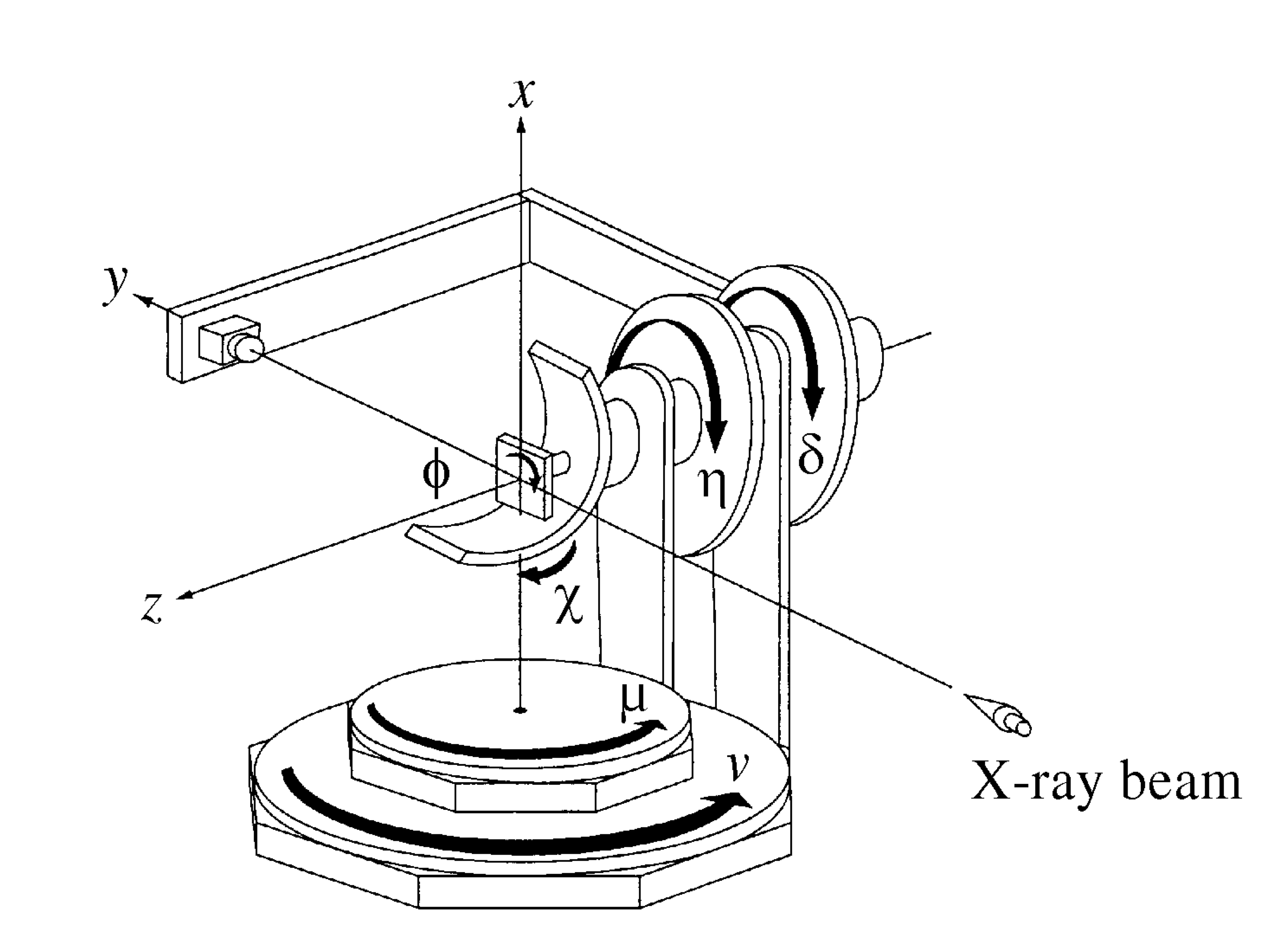
4s + 2d six-circle diffractometer, from H.You (1999)
Your Diffcalc configuration may have been customised for the geometry of your diffractometer and possibly the types of experiment you perform. For example, a five-circle diffractometer might be missing the nu circle above.
The laboratory frame is shown above. With all settings at zero as shown the crystal cartesian frame aligns with the laboratory frame. Therefor a cubic crystal mounted squarely in a way that the U matrix (defined below) is unitary will have h||a||x, k||b||y & l||c||z, crystal and reciprocal-lattice coordinate frames are defined with respect to the beam and to gravity to be (for a cubic crystal):
Overview
The following assumes that the diffractometer has been properly leveled, aligned with the beam and zeroed. See the SPEC fourc manual.
Before moving in hkl space you must calculate a UB matrix by specifying the crystal’s lattice parameters (which define the B matrix) and finding two reflections (from which the U matrix defining any mismount can be inferred); and, optionally for surface-diffraction experiments, determine how the surface of the crystal is oriented with respect to the phi axis.
Once a UB matrix has been calculated, the diffractometer may be driven in hkl coordinates. A valid diffractometer setting maps easily into a single hkl value. However for a diffractometer with more than three circles there are excess degrees of freedom when calculating a diffractometer setting from an hkl value. Diffcalc provides modes for using up the excess degrees of freedom.
Diffcalc does not perform scans directly. Instead, Scannables that use diffcalc to map between reciprocal lattice space and real diffractometer settings are scanned using the Gda’s (or minigda’s) generic scan mechanism.
Theory
Thanks to Elias Vlieg for sharing his dos based DIF software that Diffcalc
has borrowed heavily from. The version of Diffcalc described here is based on papers by
pHH. You. [You1999] and Busing & Levy [Busing1967]. (See also the THANKS.txt file.)
Getting Help
There are few commands to remember. If a command is called without arguments in some cases Diffcalc will prompt for arguments and provide sensible defaults which can be chosen by pressing enter.
Orientation. The helpub command lists all commands related with crystal
orientation and the reference vector (often used with surfaces). See the
Orientation Commands section at the end of this manual:
>>> help ub
...
HKL movement. The help hkl list all commands related to moving in reciprocal-lattice
space. See the Motion Commands section at the end of this manual:
>>> help hkl
...
Call help on any command. e.g.:
==> help loadub
Diffcalc’s Scannables
To list and show the current positions of your beamline’s scannables
use pos with no arguments:
>>> pos
Results in:
Energy and wavelength scannables:
energy    12.3984
wl:       1.0000
Diffractometer scannables, as a group and in component axes (in the real GDA these have limits):
sixc:     mu: 0.0000 delta: 0.0000 gamma: 0.0000 omega: 0.0000 chi: 0.0000 phi: 0.0000
mu:       0.0000
chi:      0.0000
delta:    0.0000
gamma:    0.0000
omega:    0.0000
phi:      0.0000
Dummy counter, which in this example simply counts at 1hit/s:
ct: 0.0000
Hkl scannable, as a group and in component:
hkl:      Error: No UB matrix
h:        Error: No UB matrix
k:        Error: No UB matrix
l:        Error: No UB matrix
Parameter scannables, used in some modes, these provide a scannable alternative to the Motion section. Some constrain of these constrain virtual angles:
alpha:    ---
beta:     ---
naz:      ---
psi:      ---
qaz:      ---
and some constrain physical angles:
phi_con:  ---
chi_con:  ---
delta_con:---
eta_con:  ---
gam_con:  ---
mu_con:   ---
Crystal orientation
Before moving in hkl space you must calculate a UB matrix by specifying the crystal’s lattice parameters (which define the B matrix) and finding two reflections (from which the U matrix can be inferred); and, optionally for surface-diffraction experiments, determine how the surface of the crystal is oriented with respect to the phi axis.
Start a new UB calculation
A UB calculation contains the description of the crystal-under-test, any saved reflections, reference angle direction, and a B & UB matrix pair if they have been calculated or manually specified. Starting a new UB calculation will clear all of these.
Before starting a UB-calculation, the ub command used to summarise
the state of the current UB-calculation, will reflect that no
UB-calculation has been started:
==> ub
A new UB-calculation calculation may be started and lattice specified explicitly:
==> newub 'example'
==> setlat '1Acube' 1 1 1 90 90 90
or interactively:
>>> newub
calculation name: example
crystal name: 1Acube
       a [1]: 1
       b [1]: 1
       c [1]: 1
  alpha [90]: 90
   beta [90]: 90
  gamma [90]: 90
where a,b and c are the lengths of the three unit cell basis vectors in Angstroms, and alpha, beta and gamma are angles in Degrees.
The ub command will show the state of the current UB-calculation
(and the current energy for reference):
==> ub
Load a UB calculation
To load the last used UB-calculation:
>>> lastub
Loading ub calculation: 'mono-Si'
To load a previous UB-calculation:
>>> listub
UB calculations in: /Users/walton/.diffcalc/i16

0) mono-Si            15 Feb 2017 (22:32)
1) i16-32             13 Feb 2017 (18:32)

>>> loadub 0
Generate a U matrix from two reflections
The normal way to calculate a U matrix is to find the position of two reflections with known hkl values. Diffcalc allows many reflections to be recorded but currently only uses the first two when calculating a UB matrix.
Find U matrix from two reflections:
==> pos wl 1
==> c2th [0 0 1]
59.99999999999999

==> pos sixc [0 60 0 30 90 0]
==> addref [0 0 1]

==> pos sixc [0 90 0 45 45 90]
==> addref [0 1 1]
Check that it looks good:
==> checkub
Manually specify U matrix
Set U matrix manually (pretending sample is squarely mounted):
==> setu [[1 0 0] [0 1 0] [0 0 1]]
Edit reflection list
Use showref to show the reflection list:
==> showref
Use swapref to swap reflections:
==> swapref 1 2
Recalculating UB matrix.
Use delref to delete a reflection:
>>> delref 1
Calculate a UB matrix
Unless a U or UB matrix has been manually specified, a new UB matrix will be calculated after the second reflection has been found, or whenever one of the first two reflections is changed.
Use the command calcub to force the UB matrix to be calculated from the
first two reflections.
If you have misidentified a reflection used for the orientation the
resulting UB matrix will be incorrect. Always use the checkub
command to check that the computed values agree with the estimated values:
==> checkub
Set the reference vector
When performing surface experiments the reference vector should be set normal to the surface. It can also be used to define other directions within the crystal with which we want to orient the incident or diffracted beam.
By default the reference vector is set parallel to the phi axis. That is, along the z-axis of the phi coordinate frame.
The ub command shows the current reference vector, along with any inferred
miscut, at the top its report (or it can be shown by calling setnphi or
setnhkl' with no args):
>>> ub
...
n_phi:      0.00000   0.00000   1.00000 <- set
n_hkl:     -0.00000   0.00000   1.00000
miscut:     None
...
The <- set label here indicates that the reference vector is set in the phi
coordinate frame. In this case, therefor, its direction in the crystal’s
reciprocal lattice space is inferred from the UB matrix.
To set the reference vector in the phi coordinate frame use:
>>> setnphi [0 0 1]
...
This is useful if the surface normal has be found with a laser or by x-ray occlusion. This vector must currently be manually calculated from the sample angle settings required to level the surface (sigma and tau commands on the way).
To set the reference vector in the crystal’s reciprocal lattice space use (this is a quick way to determine the surface orientation if the surface is known to be cleaved cleanly along a known axis):
>>> setnhkl [0 0 1] ...
Motion
Once a UB matrix has been calculated, the diffractometer may be driven in hkl coordinates. A given diffractometer setting maps easily into a single hkl value. However for a diffractometer with more than three circles there are excess degrees of freedom when calculating a diffractometer setting from an hkl value. Diffcalc provides many for using up the excess degrees of freedom.
By default Diffcalc selects no mode.
Constraining solutions for moving in hkl space
To get help and see current constraints:
>>> help con
...

==> con
Three constraints can be given: zero or one from the DET and REF columns and the
remainder from the SAMP column. Not all combinations are currently available.
Use help con to see a summary if you run into troubles.
To configure four-circle vertical scattering:
==> con gam 0 mu 0 a_eq_b
In the following the scattering plane is defined as the plane including the scattering vector, or momentum transfer vector, and the incident beam.
DETECTOR COLUMN:
- delta - physical delta setting (vertical detector motion) del=0 is equivalent to qaz=0
- gam - physical gamma setting (horizontal detector motion) gam=0 is equivalent to qaz=90
- qaz - azimuthal rotation of scattering vector (about the beam, from horizontal)
- naz - azimuthal rotation of reference vector (about the beam, from horizontal)
REFERENCE COLUMN:
- alpha - incident angle to surface (if reference is normal to surface)
- beta - exit angle from surface (if reference is normal to surface)
- psi - azimuthal rotation about scattering vector of reference vector (from scattering plane)
- a_eq_b - bisecting mode with alpha=beta. Equivalent to psi=90
SAMPLE COLUMN:
- mu, eta, chi & phi - physical settings
- mu_is_gam - force mu to follow gamma (results in a 5-circle geometry)
Diffcalc will report two other (un-constrainable) virtual angles:
- theta - half of 2theta, the angle through the diffracted beam bends
- tau - longitude of reference vector from scattering vector (in scattering plane)
Example constraint modes
There is sometimes more than one way to get the same effect.
Vertical four-circle mode:
>>> con gam 0 mu 0 a_eq_b   # or equivalently:
>>> con qaz 90 mu 0 a_eq_b

>>> con alpha 1             # replaces a_eq_b
Horizontal four-circle mode:
>>> con del 0 eta 0 alpha 1   # or equivalently:
>>> con qaz 0 mu 0 alpha 1
Surface vertical mode:
>>> con naz 90 mu 0 alpha 1
Surface horizontal mode:
>>> con naz 0 eta 0 alpha 1
Z-axis mode (surface horizontal):
>>> con chi (-sigma) phi (-tau) alpha 1
where sigma and tau are the offsets required in chi and phi to bring the surface normal parallel to eta. Alpha will determine mu directly leaving eta to orient the planes. Or:
>>> con naz 0 phi 0 alpha 1 # or any another sample angle
Z-axis mode (surface vertical):
>>> con naz 0 phi 0 alpha 1 # or any another sample angle
Changing constrained values
Once constraints are chosen constrained values may be changed directly:
==> con mu 10
or via the associated scannable:
==> pos mu_con 10
Configuring limits and cuts
Diffcalc maintains its own limits on axes. These limits will be used when choosing solutions. If more than one detector solution is exists Diffcalc will ask you to reduce the the limits until there is only one. However if more than one solution for the sample settings is available it will choose one base on heuristics.
Use the hardware command to see the current limits and cuts:
==> hardware
To set the limits:
==> setmin delta -1
==> setmax delta 145
To set a cut:
==> setcut phi -180
This causes requests to move phi to be between the configured -180 and +360 degress above this. i.e. it might dive to -10 degrees rather than 350.
Moving in hkl space
Configure a mode, e.g. four-circle vertical:
==> con gam 0 mu 0 a_eq_b
Simulate moving to a reflection:
==> sim hkl [0 1 1]
Move to reflection:
==> pos hkl [0 1 1]

==> pos sixc
Simulate moving to a location:
==> pos sixc [0 60 0 30 90 0]
Scanning in hkl space
All scans described below use the same generic scanning mechanism provided by the GDA system or by minigda. Here are some examples.
Fixed hkl scans
In a ‘fixed hkl scan’ something (such as energy or Bin) is scanned, and at each step hkl is ‘moved’ to keep the sample and detector aligned. Also plonk the diffractometer scannable (sixc) on there with no destination to monitor what is actually happening and then throw on a detector (ct) with an exposure time if appropriate:
>>> #scan scannable_name start stop step [scannable_name [pos or time]]..

>>> scan en 9 11 .5 hkl [1 0 0] sixc ct 1

>>> scan en 9 11 .5 hklverbose [1 0 0] sixc ct 1

>>> scan betain 4 5 .2 hkl [1 0 0] sixc ct 1

>>> scan alpha_par 0 10 2 hkl [1 0 0] sixc ct 1
Scanning hkl
Hkl, or one component, may also be scanned directly:
>>> scan h .8 1.2 .1 hklverbose sixc ct 1
At each step, this will read the current hkl position, modify the h component and then move to the resulting vector. There is a danger that with this method k and l may drift. To get around this the start, stop and step values may also be specified as vectors. So for example:
>>> scan hkl [1 0 0] [1 .3 0] [1 0.1 0] ct1
is equivilant to:
>>> pos hkl [1 0 0]
>>> scan k 0 .3 .1 ct1
but will not suffer from drifting. This method also allows scans along any direction in hkl space to be performed.
Multidimension scans
Two and three dimensional scans:
>>> scan en 9 11 .5 h .9 1.1 .2 hklverbose sixc ct 1
>>> scan h 1 3 1 k 1 3 1 l 1 3 1 hkl ct 1
References
| [You1999] | H. You. Angle calculations for a ‘4S+2D’ six-circle diffractometer. J. Appl. Cryst. (1999). 32, 614-623. (pdf link). |
| [Busing1967] | W. R. Busing and H. A. Levy. Angle calculations for 3- and 4-circle X-ray and neutron diffractometers. Acta Cryst. (1967). 22, 457-464. (pdf link). |